Triton Flash Attention Kernel Walkthrough: The Forward Pass

So you've learned about basic Triton language like make_block_ptr, but how does it fit into a real, high-performance GPU kernel? The best way to learn is to walk through a real-world example: a Triton implementation of FLA's highly-optimized attention mechanism, similar to FlashAttention.

This is about understanding the why—the design choices that make these kernels incredibly fast. We'll trace the execution from the high-level Python function down into the Triton kernel, explaining the GPU-specific concepts along the way.

We are not going to, however, spend time explaining basic Triton syntax. There are already resources like the official documentation which talk about them "pretty well". We will be mainly discussing the design and intuition, including small details like decorators.

Background: The FlashAttention Intuition

Standard attention has a memory problem. For a sequence of length N, it computes a massive N x N attention score matrix. For modern LLMs where N can be in the thousands, this matrix is far too large to fit in the GPU's small, ultra-fast on-chip SRAM.

This forces the GPU to constantly read and write this huge matrix to the much slower main memory (HBM or DRAM). This memory I/O, not the math, becomes the bottleneck that slows everything down.

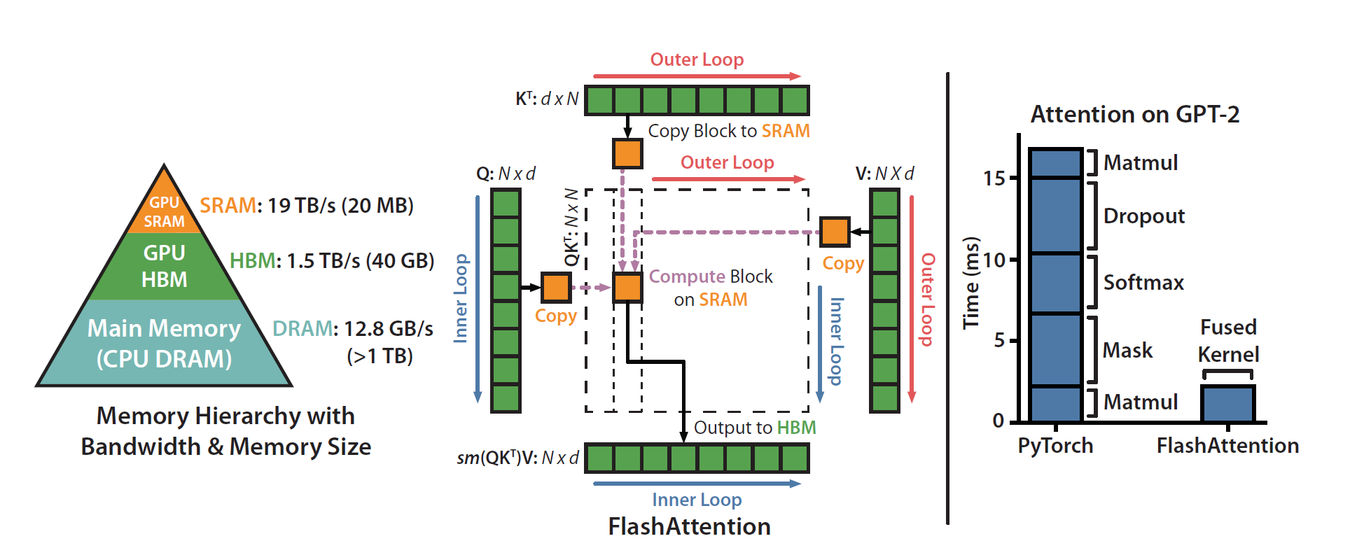
FlashAttention solves this by being I/O-aware. It redesigns the algorithm to work with the GPU's memory hierarchy:

• Tiling: Instead of computing the whole N x N matrix, FlashAttention breaks the Q, K, and V inputs into smaller blocks or "tiles." These tiles are small enough to fit in SRAM.
• On-Chip Computation: It loads a block of Q into SRAM and then iterates through the blocks of K and V. All of the expensive matrix multiplications and accumulations for these blocks happen directly within the fast SRAM, drastically reducing the data traffic to and from HBM.
• Online Softmax: A key innovation is a numerically stable "online softmax" method. It calculates the softmax normalization factor on the fly, block by block, without ever needing to see the full score matrix. This allows it to produce the exact same result as standard attention, just much, much faster.

Our Model: FlashAttention with a Twist

We will be exploring FLA's attn kernel, which uses the exact same principles of tiling and online softmax. The code is a direct implementation of this I/O-aware design.

The main difference is one added feature: an optional log-decay mechanism, controlled by a tensor g.

This allows the model to incorporate a relative positional bias into the attention scores. The calculation is modified like this:

score(q_i, k_j) = (q_i @ k_j) + (g_i - g_j)

To do this efficiently, the kernel uses a pre-computed cumulative sum of g (g_cumsum), which is loaded into SRAM along with the key and value blocks. This clever addition fits perfectly into the tiled paradigm, adding a new modeling capability without sacrificing the performance gains of FlashAttention.

With this foundation, let's trace the code from the top down.

The Big Picture: The Python Entrypoint

Everything starts with a Python function, parallel_attn. This function acts as the "mission control" before we launch our GPU code. It doesn't do any heavy computation itself; instead, its job is to prepare everything for the kernel.

def parallel_attn(
    q: torch.Tensor,
    k: torch.Tensor,
    v: torch.Tensor,
    g: Optional[torch.Tensor] = None,
    scale: Optional[float] = None,
    cu_seqlens: Optional[torch.LongTensor] = None,
    head_first: bool = False
) -> torch.Tensor:
      # 1. Handle deprecations and warnings
      # 2. Set the attention scale if not provided
      # 3. Call the autograd Function
      o = ParallelAttentionFunction.apply(q, k, v, g, scale, cu_seqlens)
      return o

This function bridges the gap between the user's PyTorch tensors and the underlying C++/CUDA-like operations. Its most important (and basically only) job is to call ParallelAttentionFunction.apply(...), which is how PyTorch's automatic differentiation system hooks into our custom code.

The autograd.Function

The ParallelAttentionFunction is the formal interface. It's a torch.autograd.Function, which requires two static methods: a forward and a backward pass. For now, we'll only focus on forward.

@torch.compile
class ParallelAttentionFunction(torch.autograd.Function):

    @staticmethod
    @contiguous
    @autocast_custom_fwd
    def forward(ctx, q, k, v, g, scale, cu_seqlens):
        ctx.dtype = q.dtype

        RCP_LN2: float = 1.4426950216
        g_cumsum = chunk_global_cumsum(g, cu_seqlens=cu_seqlens, scale=RCP_LN2) if g is not None else None
        o, lse = parallel_attn_fwd(
            q=q,
            k=k,
            v=v,
            g_cumsum=g_cumsum,
            scale=scale,
            cu_seqlens=cu_seqlens,
        )
        ctx.save_for_backward(q, k, v, o, g_cumsum, lse)
        ctx.cu_seqlens = cu_seqlens
        ctx.scale = scale
        return o.to(q.dtype)

Let's first look at the decorators. The @contiguous decorator ensures that any tensors with fragmented memory layouts (perhaps from a previous transpose operation) are made contiguous before being passed to our kernel. The @autocast_custom_fwd decorator handles mixed-precision training, a key optimization for modern GPUs. It automatically casts the input tensors to lower-precision formats like bfloat16, which allows the GPU's Tensor Cores to perform calculations much faster.

Inside the forward method, the logic is straightforward. It first performs any necessary pre-computation, like calling chunk_global_cumsum to prepare the g tensor for efficient use inside the kernel. Then, it delegates the main workload by calling parallel_attn_fwd, which is the Python function responsible for launching our Triton kernel.

Perhaps the most important job of this function is preparing for the future: the backward pass. Notice the line ctx.save_for_backward(q, k, v, o, g_cumsum, lse). The core insight of FlashAttention is that we avoid storing the massive N x N attention matrix. The price we pay for this memory saving is that we must recompute pieces of it during backpropagation. To do this, the backward pass needs the original inputs (q, k, v) and the outputs (o, lse). This line carefully packs them into the ctx, ensuring the backward pass has everything it needs to calculate the gradients efficiently.

The Launcher

parallel_attn_fwd function is the final step in our Python setup before we launch into the GPU kernel.

def parallel_attn_fwd(
    q: torch.Tensor,
    k: torch.Tensor,
    v: torch.Tensor,
    g_cumsum: torch.Tensor,
    scale: float,
    cu_seqlens: Optional[torch.LongTensor] = None,
):
    B, T, H, K, V = *k.shape, v.shape[-1]
    HQ = q.shape[2]
    G = HQ // H
    BT = 128
    # Define BS, BK, BV, and num_warps based on GPU device
    NK = triton.cdiv(K, BK)
    NV = triton.cdiv(V, BV)

    chunk_indices = prepare_chunk_indices(cu_seqlens, BT) if cu_seqlens is not None else None
    NT = triton.cdiv(T, BT) if cu_seqlens is None else len(chunk_indices)
    assert NK == 1, "The key dimension can not be larger than 256"

    o = torch.empty(B, T, HQ, V, dtype=v.dtype, device=q.device)
    lse = torch.empty(B, T, HQ, dtype=torch.float, device=q.device)
    grid = (NV, NT, B * HQ)
    parallel_attn_fwd_kernel[grid](
        q=q,
        k=k,
        v=v,
        o=o,
        g_cumsum=g_cumsum,
        lse=lse,
        scale=scale,
        cu_seqlens=cu_seqlens,
        chunk_indices=chunk_indices,
        B=B,
        T=T,
        H=H,
        HQ=HQ,
        G=G,
        K=K,
        V=V,
        BT=BT,
        BS=BS,
        BK=BK,
        BV=BV,
        num_warps=num_warps,
    )
    return o, lse

Here's a breakdown of its responsibilities:

1. Unpacking Dimensions and Handling GQA

The function begins by unpacking the shapes of the input tensors to get essential metadata like the Batch size, Time/sequence length, number of Heads, and the Key/Value dimensions. It also calculates G = HQ // H, which is the key to handling Grouped-Query Attention (GQA). GQA is an optimization where multiple query heads (HQ) can share a single key/value head (H) to save memory bandwidth and computation, and this G factor tells the kernel how many query heads belong to each group.

2. Defining Hardware-Specific Block Sizes

Next, the tile sizes (BS, BK, BV) and num_warps are set based on the GPU architecture (e.g., Hopper, Ampere). Different GPU generations have different amounts of fast SRAM and different memory architectures. This code chooses the optimal block sizes to maximize performance—a larger, more powerful GPU can handle bigger chunks of data at once.

3. Calculating the Grid Dimensions

With the block sizes defined, the function calculates how many blocks are needed to cover the entire problem space. NV = triton.cdiv(V, BV) calculates the number of blocks needed for the value dimension, while NT = triton.cdiv(T, BT) does the same for the time dimension.

4. Allocating Output Tensors

The function then pre-allocates the memory for the final outputs by calling torch.empty. o is the main output tensor, and lse is the log-sum-exp tensor, which stores the softmax normalization factor needed for a stable backward pass. By creating these tensors in PyTorch beforehand, we provide the Triton kernel with pointers to the exact memory locations where it should write its results.

5. Defining and Launching the Grid

This is the final, most important step. The grid = (NV, NT, B * HQ) tuple defines the 3D shape of our parallel execution, specifying that we will launch a swarm of NV * NT * (B * HQ) independent programs. The call parallel_attn_fwd_kernel[grid](...) is Triton's unique syntax for launching this grid.

Inside the Kernel: parallel_attn_fwd_kernel

Finally, the Triton kernel itself. While it looks like Python, this function is compiled by Triton into highly optimized machine code that runs in parallel across thousands of GPU threads.

@triton.heuristics({
    'USE_G': lambda args: args['g_cumsum'] is not None,
    'IS_VARLEN': lambda args: args['cu_seqlens'] is not None,
})
@triton.jit
def parallel_attn_fwd_kernel(
    q,
    k,
    v,
    o,
    g_cumsum,
    lse,
    scale,
    cu_seqlens,
    chunk_indices,
    T,
    B: tl.constexpr,
    H: tl.constexpr,
    HQ: tl.constexpr,
    G: tl.constexpr,
    K: tl.constexpr,
    V: tl.constexpr,
    BT: tl.constexpr,
    BS: tl.constexpr,
    BK: tl.constexpr,
    BV: tl.constexpr,
    USE_G: tl.constexpr,
    IS_VARLEN: tl.constexpr,
):
    i_v, i_t, i_bh = tl.program_id(0), tl.program_id(1), tl.program_id(2)
    i_b, i_hq = i_bh // HQ, i_bh % HQ
    i_h = i_hq // G

    if IS_VARLEN:
        i_n, i_t = tl.load(chunk_indices + i_t * 2).to(tl.int32), tl.load(chunk_indices + i_t * 2 + 1).to(tl.int32)
        bos, eos = tl.load(cu_seqlens + i_n).to(tl.int32), tl.load(cu_seqlens + i_n + 1).to(tl.int32)
        T = eos - bos
    else:
        i_n = i_b
        bos, eos = i_n * T, i_n * T + T
    RCP_LN2: tl.constexpr = 1.4426950216

    p_q = tl.make_block_ptr(q + (bos * HQ + i_hq) * K, (T, K), (HQ*K, 1), (i_t * BT, 0), (BT, BK), (1, 0))
    p_o = tl.make_block_ptr(o + (bos * HQ + i_hq) * V, (T, V), (HQ*V, 1), (i_t * BT, i_v * BV), (BT, BV), (1, 0))
    p_lse = tl.make_block_ptr(lse + bos * HQ + i_hq, (T,), (HQ,), (i_t * BT,), (BT,), (0,))

    # the Q block is kept in the shared memory throughout the whole kernel
    # [BT, BK]
    b_q = tl.load(p_q, boundary_check=(0, 1))
    # [BT, BV]
    b_o = tl.zeros([BT, BV], dtype=tl.float32)

    b_m = tl.full([BT], float('-inf'), dtype=tl.float32)
    b_acc = tl.zeros([BT], dtype=tl.float32)

    if USE_G:
        p_g = tl.make_block_ptr(g_cumsum + bos * HQ + i_hq, (T,), (HQ,), (i_t * BT,), (BT,), (0,))
        b_gq = tl.load(p_g, boundary_check=(0,)).to(tl.float32)
    else:
        b_gq = None

    for i_s in range(0, i_t * BT, BS):
        p_k = tl.make_block_ptr(k + (bos * H + i_h) * K, (K, T), (1, H*K), (0, i_s), (BK, BS), (0, 1))
        p_v = tl.make_block_ptr(v + (bos * H + i_h) * V, (T, V), (H*V, 1), (i_s, i_v * BV), (BS, BV), (1, 0))
        # [BK, BS]
        b_k = tl.load(p_k, boundary_check=(0, 1))
        # [BS, BV]
        b_v = tl.load(p_v, boundary_check=(0, 1))
        # [BT, BS]
        b_s = tl.dot(b_q, b_k) * scale * RCP_LN2

        if USE_G:
            o_k = i_s + tl.arange(0, BS)
            m_k = o_k < T
            b_gk = tl.load(g_cumsum + (bos + o_k) * HQ + i_hq, mask=m_k, other=0).to(tl.float32)
            b_s += b_gq[:, None] - b_gk[None, :]

        # [BT, BS]
        b_m, b_mp = tl.maximum(b_m, tl.max(b_s, 1)), b_m
        b_r = exp2(b_mp - b_m)
        # [BT, BS]
        b_p = exp2(b_s - b_m[:, None])
        # [BT]
        b_acc = b_acc * b_r + tl.sum(b_p, 1)
        # [BT, BV]
        b_o = b_o * b_r[:, None] + tl.dot(b_p.to(b_q.dtype), b_v)

        b_mp = b_m

    # [BT]
    o_q = i_t * BT + tl.arange(0, BT)
    for i_s in range(i_t * BT, min((i_t + 1) * BT, T), BS):
        p_k = tl.make_block_ptr(k + (bos * H + i_h) * K, (K, T), (1, H*K), (0, i_s), (BK, BS), (0, 1))
        p_v = tl.make_block_ptr(v + (bos * H + i_h) * V, (T, V), (H*V, 1), (i_s, i_v * BV), (BS, BV), (1, 0))

        # [BS]
        o_k = i_s + tl.arange(0, BS)
        m_k = o_k < T
        # [BK, BS]
        b_k = tl.load(p_k, boundary_check=(0, 1))
        # [BS, BV]
        b_v = tl.load(p_v, boundary_check=(0, 1))
        # [BT, BS]
        b_s = tl.dot(b_q, b_k) * scale * RCP_LN2

        if USE_G:
            b_gk = tl.load(g_cumsum + (bos + o_k) * HQ + i_hq, mask=m_k, other=0).to(tl.float32)
            b_s += b_gq[:, None] - b_gk[None, :]

        b_s = tl.where((o_q[:, None] >= o_k[None, :]) & m_k[None, :], b_s, float('-inf'))

        # [BT]
        b_m, b_mp = tl.maximum(b_m, tl.max(b_s, 1)), b_m
        b_r = exp2(b_mp - b_m)
        # [BT, BS]
        b_p = exp2(b_s - b_m[:, None])
        # [BT]
        b_acc = b_acc * b_r + tl.sum(b_p, 1)
        # [BT, BV]
        b_o = b_o * b_r[:, None] + tl.dot(b_p.to(b_q.dtype), b_v)
        b_mp = b_m

    b_o = b_o / b_acc[:, None]
    b_m += log2(b_acc)
    tl.store(p_o, b_o.to(p_o.dtype.element_ty), boundary_check=(0, 1))
    tl.store(p_lse, b_m.to(p_lse.dtype.element_ty), boundary_check=(0,))

@triton.heuristics

At the top, the @triton.heuristics creates compile-time boolean flags like USE_G and IS_VARLEN based on the function's arguments. This allows Triton to generate specialized versions of the kernel for each case which removes the overhead of checking these conditions at runtime.

Set up

The first thing each program does is get its unique assignment from the grid using tl.program_id. This gives it the coordinates (i_v, i_t, i_bh) for the specific output tile it needs to compute. It also handles the logic for variable-length sequences, looking up the correct start (bos) and end (eos) positions if needed.

This trick of deriving bos and eos from cu_seqlen can very conveniently distinguish fixed length and varlen cases while allowing them to use the same kernels - it's a common practice in FLA!

Next, a block of the query tensor, b_q, is loaded into the fast on-chip SRAM just once. This query block will be reused repeatedly against all relevant key blocks, which is a core principle of maximizing computational intensity.

Notice how, when you are loading the tensors using make_block_ptr, that you don't pass the stride parameter explicitly (which is what most codes do). This is because the striding variables can actually be very easily calculated, and it makes the code cleaner!

Finally, the kernel initializes three crucial "accumulator" variables in SRAM: b_o (the output), b_m (the running maximum score, for numerical stability), and b_acc (the running denominator for the softmax).

The Main Loop

The kernel then enters its main loop, iterating through blocks of the key and value tensors. The logic here is a direct implementation of the FlashAttention algorithm. For each block, it performs these steps:

1. It uses tl.make_block_ptr to create views for the current key and value tiles and tl.load to bring them into fast SRAM. Note the use of the "virtual transpose" trick (order parameter in make_block_ptr) for p_k to efficiently load a tile ready for the dot product.
2. It calculates the attention scores for the current tiles using the highly optimized tl.dot instruction, which maps to the GPU's Tensor Cores. If the decay g is used, its value is added to the scores here.
3. This is the "online" part of the algorithm. It updates the running maximum b_m and uses it to rescale the current accumulators b_o and b_acc before adding in the new values. This is a numerically stable way to compute softmax without seeing all the scores at once.

The Diagonal Block and Finalization

After processing all the previous blocks, the kernel has a special loop to handle the "diagonal" block, where the query and key indices overlap. Here, it applies a causal mask using tl.where to ensure that a query at a given position can only attend to keys at or before that position.

It is using two separate loops instead of one because this avoids using tl.where, a slow operation, for every chunk of the sequence.

Once all blocks have been processed, the kernel performs the final normalization: b_o is divided by the final accumulator b_acc. The log-sum-exp value (lse), which is needed for the backward pass, is also calculated. Finally, tl.store writes these finished results from the fast SRAM back into the main global memory, completing the program's assignment.

More to come

While attention is a critical component, it is just one of many computational primitives that benefit from this level of optimization. Similar deep dives are possible for operations ranging from specialized convolutions and fused activation functions to custom optimizer steps.

Understanding the implementation details of these core operational layers provides a deeper insight than architectural diagrams alone. And every ML algorithms should be hardware-aligned!