Matrix Multiplication and Memory

Before diving into Triton kernels or any optimization tricks, I think it's worth grounding the discussion in what we're actually trying to speed up: matrix multiplication. If you're already familiar with the basics, feel free to jump to the next part. This part is more about setting the stage for why things get complicated on a GPU.

Matrix multiplication is probably one of the most straightforward operations to write down but deceptively hard to optimize. You take two matrices, say $A$ of shape $(M, K)$ and $B$ of shape $(K, N)$, and you want to compute $C = AB$ of shape $(M, N)$. Each element $C_{ij}$ is a dot product between the $i$-th row of $A$ and the $j$-th column of $B$. That's it. One loop over rows, one over columns, and one over the inner dimension $K$ for the dot product:

# Simple matrix multiplication
for i in range(M):
    for j in range(N):
        for k in range(K):
            C[i][j] += A[i][k] * B[k][j]

But that triple for-loop is exactly what we want to avoid, especially on a GPU.

Jumping back to hardware for a second. Unlike other languages, when I started looking into Triton, different hardware-related terms kept coming up (e.g. DRAM, SRAM, etc.) I vaguely knew GPUs had different types of memory, but I hadn't internalized what that meant. So here's what I learned, put concisely.

GPUs have a memory hierarchy. DRAM, or global memory, is huge (e.g. 10GB) but slow. Accessing DRAM takes hundreds of clock cycles. On the other hand, there's SRAM, which is super fast (a few cycles), but tiny (typically just tens of kilobytes per thread block). This SRAM is also called shared memory, and using it well is one of the biggest goals in GPU programming, which is why FlashAttention was so useful.

Now imagine if we actually ran that triple for-loop above on the GPU, naïvely. Every access to A[i][k] or B[k][j] would go to DRAM, which is a lot of memory traffic. Worse, the same values would get read over and over again by different threads, wasting bandwidth. So even though the GPU has hundreds of threads ready to compute some numbers, they end up waiting around for memory. That's the bottleneck—not compute, but memory.

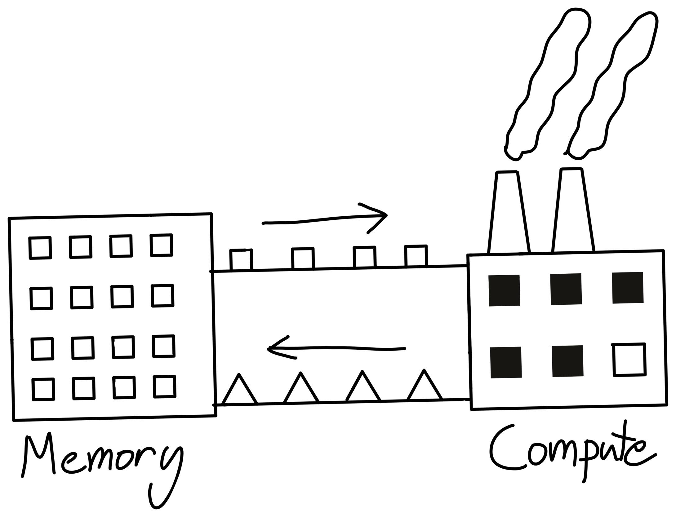
This is a figure taken from Horace's blog. Despite the fast speed of "Compute", it still has to wait for "Memory" to send over the data.

This is where things started to click for me. If DRAM is the bottleneck, then optimization is basically a game of reducing DRAM reads. The idea is to read chunks of the matrices into faster SRAM, reuse them as much as possible, and only go back to DRAM when we have to.

So instead of computing the entire matrix product, we do it in blocks. We divide $C$ into tiles as $C_{tile}$, and compute each tile in parallel. For each tile, we load a sub-block of $A$ and a sub-block of $B$ into SRAM, do the partial product, and accumulate the result.

# Tiled matrix multiplication
for m in range(0, M, BLOCK_SIZE_M):  # Parallel
    for n in range(0, N, BLOCK_SIZE_N):  # Parallel
        acc = zeros((BLOCK_SIZE_M, BLOCK_SIZE_N), dtype=float32)
        for k in range(0, K, BLOCK_SIZE_K):
            a = A[m:m+BLOCK_SIZE_M, k:k+BLOCK_SIZE_K]
            b = B[k:k+BLOCK_SIZE_K, n:n+BLOCK_SIZE_N]
            acc += dot(a, b)
        C[m:m+BLOCK_SIZE_M, n:n+BLOCK_SIZE_N] = acc

Memory Access in Triton

Continuing from the tiled matmul structure, the idea is that each GPU thread (or program, in Triton terms) is responsible for one output tile of $C$. But unlike NumPy, where we can just slice a matrix and trust the high-level abstraction to find the data for us, Triton makes us explicitly tell the hardware where in memory to look. We do this by using pointers.

So here's what's actually happening.

In the GPU, matrices like $A$ and $B$ are stored in memory as giant, flat 1d arrays. There's no A[i][j] concept at the hardware level. To load a tile of matrix $A$, we have to compute the address of each element in that tile manually. That's where strides come in.

Suppose matrix $A$ has shape $(M, K)$, and it's laid out row-major. The stride stride_am tells us how far we need to move in memory to go from one row to the next (usually just K), and stride_ak tells us how far to move to go from one column to the next (usually 1).

Now, each Triton program gets a program ID (pid_m, pid_n) that identifies which output tile of $C$ it's supposed to compute. So if I'm the program handling tile $(m, n)$, I need to fetch the right part of $A$ (rows starting at m) and the right part of $B$ (columns starting at n).

When written in Triton (import triton.language as tl), it can be shown as:

# Calculate offset indices for matrices
offs_am = (pid_m * BLOCK_SIZE_M + tl.arange(0, BLOCK_SIZE_M)) % M
offs_bn = (pid_n * BLOCK_SIZE_N + tl.arange(0, BLOCK_SIZE_N)) % N
offs_k = tl.arange(0, BLOCK_SIZE_K)

# Calculate memory pointers
a_ptrs = a_ptr + (offs_am[:, None] * stride_am + offs_k[None, :] * stride_ak)
b_ptrs = b_ptr + (offs_k[:, None] * stride_bk + offs_bn[None, :] * stride_bn)

Here, tl.arange(0, BLOCK_SIZE_M) gives a vector [0, 1, 2, ..., BLOCK_SIZE_M - 1], representing the offsets within a tile. Multiplying pid_m * BLOCK_SIZE_M tells us where this tile starts globally. The sum gives us the actual global row indices we're responsible for. The modulo just ensures we don't go out of bounds.

Same logic applies to columns of $B$ (via offs_bn), and offs_k handles the shared K dimension that we iterate over in the innermost loop.

So now we know which row indices to pull from $A$ and which column indices from $B$, but we still need to turn those indices into actual memory addresses. Here's how that works:

a_ptrs = a_ptr + (offs_am[:, None] * stride_am + offs_k[None, :] * stride_ak)
b_ptrs = b_ptr + (offs_k[:, None] * stride_bk + offs_bn[None, :] * stride_bn)

This part took me a while to really internalize. These expressions are essentially doing a broadcasted 2D addition to compute the addresses of each element in the (BLOCK_SIZE_M, BLOCK_SIZE_K) and (BLOCK_SIZE_K, BLOCK_SIZE_N) tiles of $A$ and $B$. Think of it like building a coordinate grid of pointers.

offs_am[:, None] * stride_am gives us a column vector of row strides, and offs_k[None, :] * stride_ak gives us a row vector of column strides. When we add them together, we get a matrix of memory offsets corresponding to each element in the tile. Adding this to the base pointer gives us the actual addresses in DRAM.

Same thing goes for b_ptrs. The only difference is that we transpose the broadcast, since the tile of $B$ is shaped the other way around.

Then, in the inner loop over k, we want to move to the next chunk of $K$ entries. That's done with:

# Update pointers to next block
a_ptrs += BLOCK_SIZE_K * stride_ak
b_ptrs += BLOCK_SIZE_K * stride_bk

These lines just advance our pointers along the $K$ axis.

Here I think the essence behind Triton is shown pretty clearly. It's not that Triton is lower is lower level than PyTorch, but more like you being closer to the metal. You can directly tell the hardware what to do, which, I have to admit, is hard at first (I'm still on day 3). But this is also kind of elegant :)

So now we've got our pointers. We've told the program which elements to load. The next step is loading them into SRAM, masking out-of-bound values, and doing the actual dot product.

The Triton code for the above methodology can be implemented as follows:

@triton.jit
def matmul(a_ptr, b_ptr, c_ptr, stride_am, stride_ak, stride_bn, stride_bk,
           BLOCK_SIZE_M, BLOCK_SIZE_N, BLOCK_SIZE_K, N, M, K):
    
    pid = tl.program_id(axis=0)
    grid_n = tl.cdiv(N, BLOCK_SIZE_N)
    pid_m = pid // grid_n
    pid_n = pid % grid_n
    
    # Calculate offset indices for matrices
    offs_am = (pid_m * BLOCK_SIZE_M + tl.arange(0, BLOCK_SIZE_M)) % M
    offs_bn = (pid_n * BLOCK_SIZE_N + tl.arange(0, BLOCK_SIZE_N)) % N
    offs_k = tl.arange(0, BLOCK_SIZE_K)
    
    # Calculate memory pointers
    a_ptrs = a_ptr + (offs_am[:, None] * stride_am + offs_k[None, :] * stride_ak)
    b_ptrs = b_ptr + (offs_k[:, None] * stride_bk + offs_bn[None, :] * stride_bn)
    
    # Initialize accumulator
    acc = tl.zeros((BLOCK_SIZE_M, BLOCK_SIZE_N), dtype=tl.float32)
    
    # Perform the matrix multiplication
    for k_ptr in tl.range(0, K, BLOCK_SIZE_K):
        a = tl.load(a_ptrs, mask=(offs_am[:, None] < M), other=0.0)
        b = tl.load(b_ptrs, mask=(offs_bn[None, :] < N), other=0.0)
        acc += tl.dot(a, b)
        
        # Update pointers to next block
        a_ptrs += BLOCK_SIZE_K * stride_ak
        b_ptrs += BLOCK_SIZE_K * stride_bk
    
    # Store the result
    c_ptrs = c_ptr + (offs_am[:, None] * stride_am + offs_bn[None, :] * stride_bn)
    mask_c = (offs_am[:, None] < M) & (offs_bn[None, :] < N)
    tl.store(c_ptrs, acc, mask=mask_c)

Directly interpreting every line one-shot can be stressful, a great resource to use here is the official Triton language documentation.

L2 Cache Optimizations

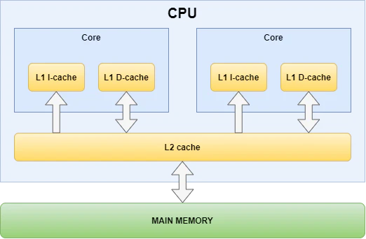
By this point, the program has already done three things: tile the matrices, calculate memory pointers manually, and iterate through blocks along the $K$ dimension. But performance on a GPU often relies on one more thing: memory access patterns. Specifically, how effectively we use the L2 cache—a layer of memory that sits between the slow global memory (DRAM) and the fast, limited SRAM (shared memory)—can significantly affect throughput.

L2 Cache Hit Rate

Each time a Triton program reads data from global memory, the hardware will first check whether that data is already available in the L2 cache. If so, it can be fetched quickly. If not, the request travels out to DRAM, which incurs far higher latency and bandwidth cost. The percentage of reads satisfied by the cache here is the L2 cache hit rate. A high L2 cache hit rate is therefore critical for maintaining high throughput, especially when multiple programs are accessing overlapping regions of the same matrix.

By saying how multiple programs are accessing "overlapping regions of the same matrix", I'm referring to them as sharing the same tile from the original matrix to fetch on. Suppose several programs are working on different row tiles of $C$, the final output, but all require access to the same block of $B$, then you can group those programs together to run faster. On the other hand, if they instead use scattered rows of $A$ that don't fit neatly into nearby memory regions. then those reads can become redundant and expensive, which will significantly slow the system down.

To address this, Triton allows you to reorder program IDs so that threads working on spatially adjacent tiles of $C$ are launched in a way that encourages temporal and spatial locality. The technique is often called grouped ordering or grouped tiling.

Here is how this logic typically looks:

# L2 Cache optimization group logic
pid = tl.program_id(axis=0)
num_pid_m = tl.cdiv(M, BLOCK_SIZE_M)
num_pid_n = tl.cdiv(N, BLOCK_SIZE_N)
num_pid_in_group = GROUP_SIZE_M * num_pid_n
group_id = pid // num_pid_in_group
first_pid_m = group_id * GROUP_SIZE_M
group_size_m = min(num_pid_m - first_pid_m, GROUP_SIZE_M)
pid_m = first_pid_m + ((pid % num_pid_in_group) % group_size_m)
pid_n = (pid % num_pid_in_group) // group_size_m

This mapping groups program IDs along the $M$ dimension (across rows of $A$) so that a contiguous group of program instances processes neighboring row tiles before moving on to distant rows. The hope here is that when one group reads a particular chunk of $A$, that data remains in the L2 cache just long enough for the next nearby program to reuse it. The same principle applies for $B$ if the $N$ axis is also grouped accordingly.

While this remapping does not change the mathematical correctness of the kernel, it does improve data reuse at the memory hierarchy level. This optimization is not always necessary, but in practice, especially for large matrices or when memory bandwidth becomes the bottleneck, grouping can increase L2 cache hit rates dramatically.

Implementation Example

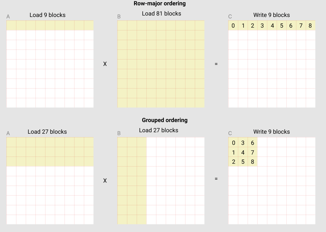
Here's a nice example taken from the original tutorial documentation:

In the following matmul where each matrix is 9 blocks by 9 blocks, we can see that if we compute the output in row-major ordering, we need to load 90 blocks into SRAM to compute the first 9 output blocks, but if we do it in grouped ordering, we only need to load 54 blocks.

This is the heart of L2 cache optimization, and now we can write the full new form:

@triton.jit
def matmul_kernel(
        # Pointers and dimensions
        a_ptr, b_ptr, c_ptr, M, N, K,
        # Strides
        stride_am, stride_ak, stride_bk, stride_bn, stride_cm, stride_cn,
        # Meta-parameters
        BLOCK_SIZE_M: tl.constexpr, BLOCK_SIZE_N: tl.constexpr, 
        BLOCK_SIZE_K: tl.constexpr, GROUP_SIZE_M: tl.constexpr,
):
    # Group mapping logic (for L2 cache optimization)
    pid = tl.program_id(axis=0)
    num_pid_m = tl.cdiv(M, BLOCK_SIZE_M)
    num_pid_n = tl.cdiv(N, BLOCK_SIZE_N)
    num_pid_in_group = GROUP_SIZE_M * num_pid_n
    group_id = pid // num_pid_in_group
    pid_m_start = group_id * GROUP_SIZE_M
    group_size_m = min(GROUP_SIZE_M, num_pid_m - pid_m_start)
    pid_m = pid_m_start + ((pid % num_pid_in_group) % group_size_m)
    pid_n = (pid % num_pid_in_group) // group_size_m
    
    # Calculate offset indices and pointers
    offs_m = pid_m * BLOCK_SIZE_M + tl.arange(0, BLOCK_SIZE_M)
    offs_n = pid_n * BLOCK_SIZE_N + tl.arange(0, BLOCK_SIZE_N)
    offs_k = tl.arange(0, BLOCK_SIZE_K)
    a_ptrs = a_ptr + (offs_m[:, None] * stride_ak + offs_k[None, :] * stride_am)
    b_ptrs = b_ptr + (offs_k[:, None] * stride_bk + offs_n[None, :] * stride_bn)
    
    # Matrix multiplication
    acc = tl.zeros((BLOCK_SIZE_M, BLOCK_SIZE_N), dtype=tl.float32)
    for k in range(0, tl.cdiv(K, BLOCK_SIZE_K)):
        # Load blocks with masks for out-of-bounds
        a = tl.load(a_ptrs, mask=offs_k[None, :] < K - k * BLOCK_SIZE_K, other=0.0)
        b = tl.load(b_ptrs, mask=offs_k[:, None] < K - k * BLOCK_SIZE_K, other=0.0)
        # Multiply and accumulate
        acc += tl.dot(a, b)
        # Advance pointers
        a_ptrs += BLOCK_SIZE_K * stride_ak
        b_ptrs += BLOCK_SIZE_K * stride_bk
        
    # Convert to float16 for output
    c = acc.to(tl.float16)
    
    # Store result with mask for out-of-bounds
    offs_cm = pid_m * BLOCK_SIZE_M + tl.arange(0, BLOCK_SIZE_M)
    offs_cn = pid_n * BLOCK_SIZE_N + tl.arange(0, BLOCK_SIZE_N)
    c_ptrs = c_ptr + stride_cm * offs_cm[:, None] + stride_cn * offs_cn[None, :]
    c_mask = (offs_cm[:, None] < M) & (offs_cn[None, :] < N)
    tl.store(c_ptrs, c, mask=c_mask)

We can now create a convenience wrapper function that only takes two input tensors, and (1) checks any shape constraint; (2) allocates the output; (3) launches the above kernel.

def matmul(a, b):
    # Check constraints and allocate output
    M, K = a.shape
    K, N = b.shape
    c = torch.empty((M, N), device=a.device, dtype=torch.float16)
    
    # Launch kernel
    grid = lambda META: (triton.cdiv(M, META['BLOCK_SIZE_M']) * 
                         triton.cdiv(N, META['BLOCK_SIZE_N']), )
    matmul_kernel[grid](
        a, b, c, M, N, K,
        a.stride(0), a.stride(1), b.stride(0), b.stride(1), 
        c.stride(0), c.stride(1),
    )
    return c

To this point, the tutorial has come to an end. I don't think this tutorial comprehensively covered everything one needs to understand matmul in Triton (e.g. I did not cover the basic language syntax). When I was learning on my own, I turned to a great amount of tutorials and q&as with gpt, so my purpose for writing this blog is rather to provide a starting point of understanding the field. Right now when I'm typing these letters down, I'm also just on day 3 of learning Triton from scratch!

The tutorial documentation is a great place to visit next.